

Experiments with a high-pressure capillary rheometer are often the only way to determine the viscosity at higher, process-relevant shear rates. The measuring principle requires different corrections to be made to get true shear rate and shear stress. When these corrections are made, reliable viscosity data can be obtained. So-called apparent data is converted into true material property data. Which corrections are actually necessary depends on the individual application. The correct order in which these corrections are made, also plays an important role and will be discussed in the last chapter of this paper.
Basic Equations - Apparent Values
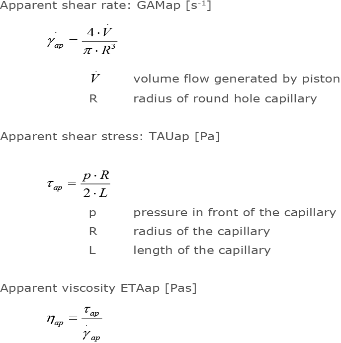
Raw data used: Pressure, or piston force before the capillary, piston speed, geometry data of the piston and capillary. Using this input, the apparent values are calculated first. For the round hole capillary, the formulas are:
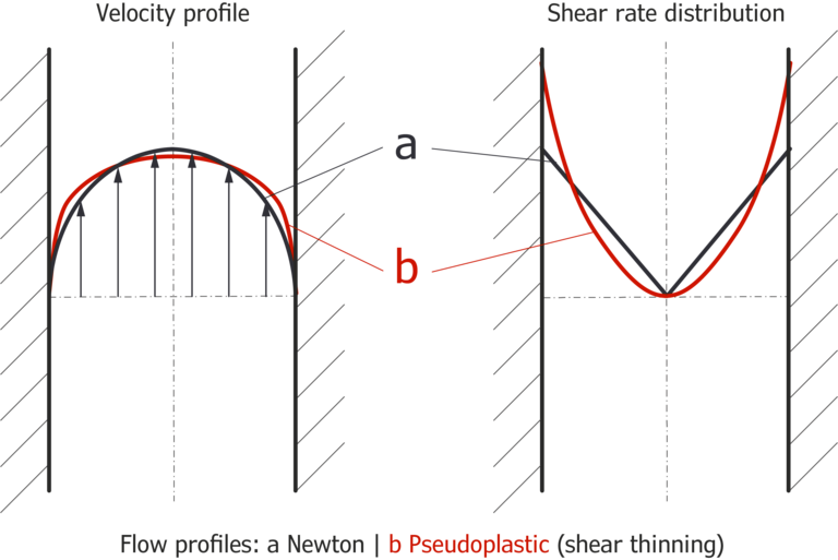
As a result of shear thinning in real polymer melts with pseudoplastic flow behavior, there is a strong curvature of the velocity profile towards the wall. As a result, shear rates on the wall are increased over the Newtonian medium.
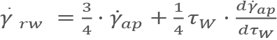
During the experiment, Newtonian behavior is assumed for the calculation of the apparent shear rate. The correction of the apparent shear rate, according to Weißenberg-Rabinowitsch, for round-hole capillaries is:
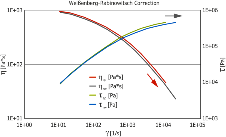
The Weißenberg-Rabinowitsch correction assumes pseudo plastic behavior of the material when correcting shear rates of the different measuring points, especially at higher shear rates. As a result, the viscosity is shifted as shown in the following diagram.
The pressure measurement is typically done above the capillary in the test barrel. As a result, in addition to the viscous pressure loss, measurements also include losses measured due to inlet and outlet effects.
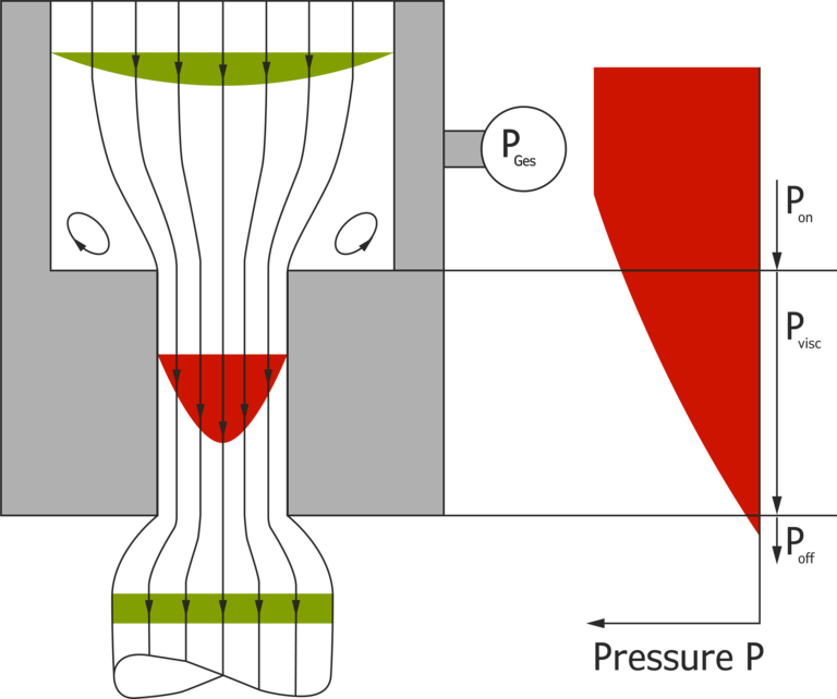
Using the Bagley correction, the viscous pressure drop in the capillary is separated from the pressure losses due to run-in and run-out effects.
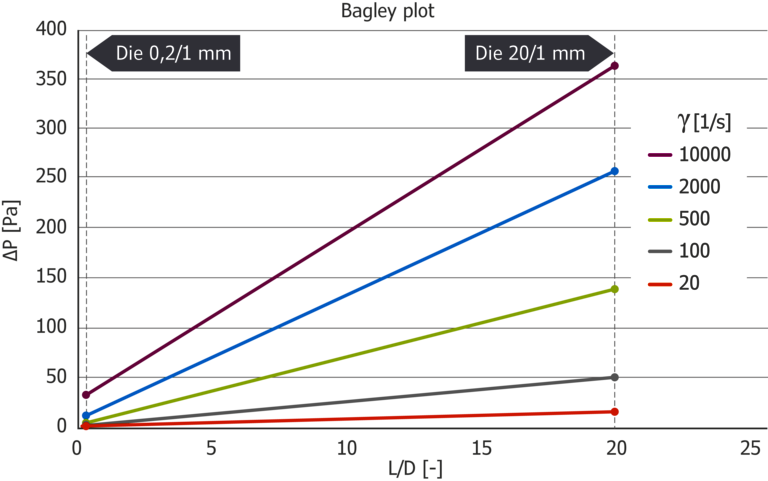
To determine the inlet-outlet pressure loss, the pressure loss is plotted for different capillaries of the same diameter, but with different lengths and extrapolated to zero (Bagley plot). Before the evaluation, at least two measurements with capillaries of the same diameter, but different lengths, must be carried out. It is essential that the shortest capillary is not too far from zero in length and the capillary lengths are not too close together to avoid extrapolation errors.
A practical combination for the linear Bagley correction is given by using the capillaries L/D=30/1 mm, 20/1 mm and 10/1 mm.
A favorable combination for a nonlinear Bagley correction is given by using the capillaries L/D=20/1 mm, L/D=10/1 mm and L/D=5/1 mm.
If the inlet pressure loss is determined with only two capillaries, the combination L/D=20/1 mm and L/D=0.2/1 mm is favorable. However, nonlinearities cannot be detected. The following diagram shows a Bagley plot with this combination of capillaries.
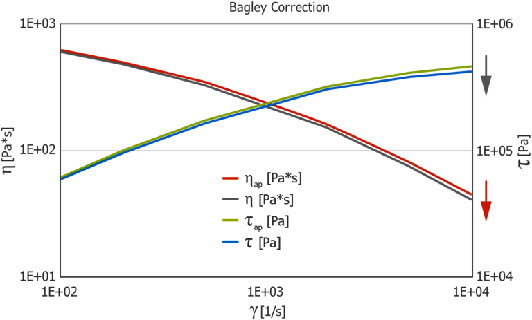
Shear stress as well as viscosity is corrected downwards by Bagley correction.
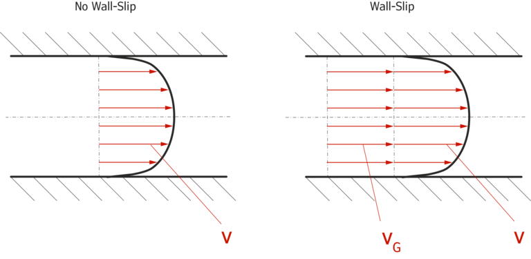
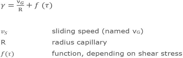
Mooney Correction is used to determine the wall slip rate for wall-slip materials, such as wall-sliding materials like HDPE or PVC. The model assumes that the material with constant wall slip speed vg is slipping at the wall.
Integration via the velocity profile yields the following relationship for the shear rate:
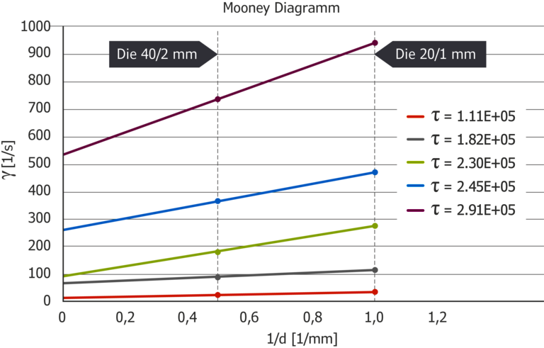
Due to this correlation, measurements at constant shear stress have to be made with capillaries of different diameter, but with the same L/D ratio. A practical die combination for the linear Mooney correction is using capillaries such as L/D=40/2 mm and L/D=20/1 mm.
Measurements taken at constant speed can also be calculated using the Mooney correction. Thereby points with the same shear stress are automatically determined by interpolation. When setting up the measurement, the piston speed at different shear rates has to be adjusted.
The result shows the Mooney diagram with shear rates above the reciprocal diameter. The slope angle of the straight line in the diagram gives the wall slip speed.
The following Mooney diagram shows data from measurements with the capillary pair L/D=40/2 mm and L/D=20/1 mm. Shear rate at constant shear stress is plotted against the reciprocal capillary diameter. The function of shear stress ⨍(τ) thus becomes the constant y-axis section and the sliding velocity VG can be determined from the slope of the straight line.
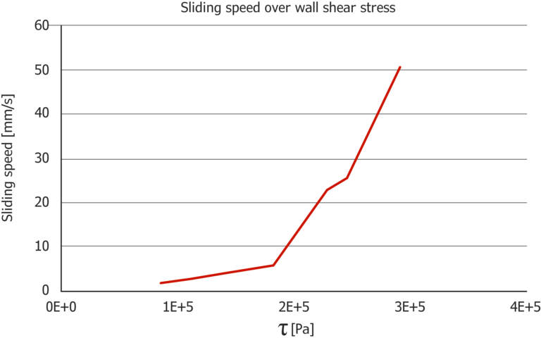
Technologically interesting is the plot of shear rate versus shear stress. Here, the so-called critical shear stress can be determined, at which wall slip occurs.
Furthermore, areas of the shear stress can be detected, in which high slipping speeds or large changes in the slipping speed occur. Choosing to operate in the range of this shear stress can lead to instabilities in the process due to the wildly changing, or high slipping speeds.
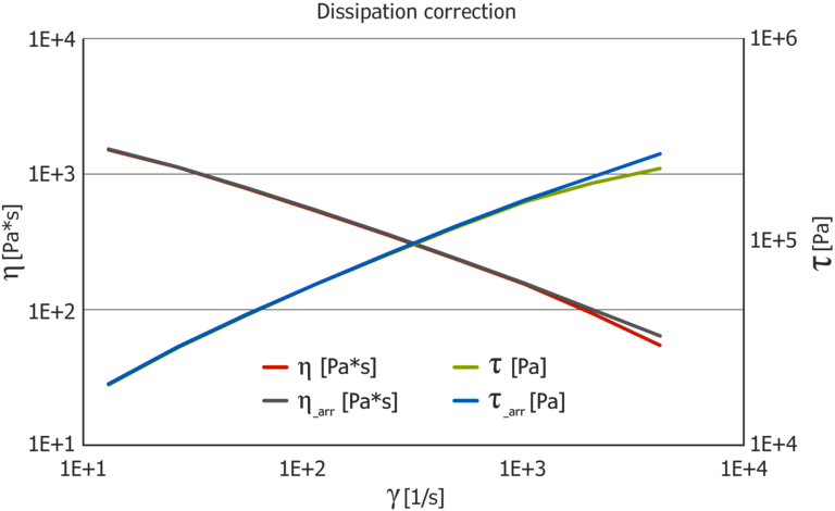
The pressure loss that occurs when flowing through the capillary leads to an increase in temperature in the capillary. Also, when the material is redirected into the smaller capillary itself, this creates friction heat. The resulting temperature increase is determined by the FeCo thermocouple plugged into the steel wall of the actual capillary.
The Arrhenius temperature shift calculates the viscosity back to the current steel temperature (=setpoint temperature).

Such a correction is necessary, especially at high shear rates. At shear rates of 10.000 1/s and more, temperatures may increase 5-10 °C or more, depending on the test material.
The resulting corrections for thermoplastics are in the range of 10 % or more, but can be significantly higher in the case of elastomers. In order to perform the dissipation correction, the activation energy EA of the sample must be known.
This can be determined by making three viscosity measurements at different temperatures and using the temperature shift function of the software. The following diagram shows the effect of the dissipation correction. Both shear stress and viscosity are converted at the high shear rates to the setpoint temperature.
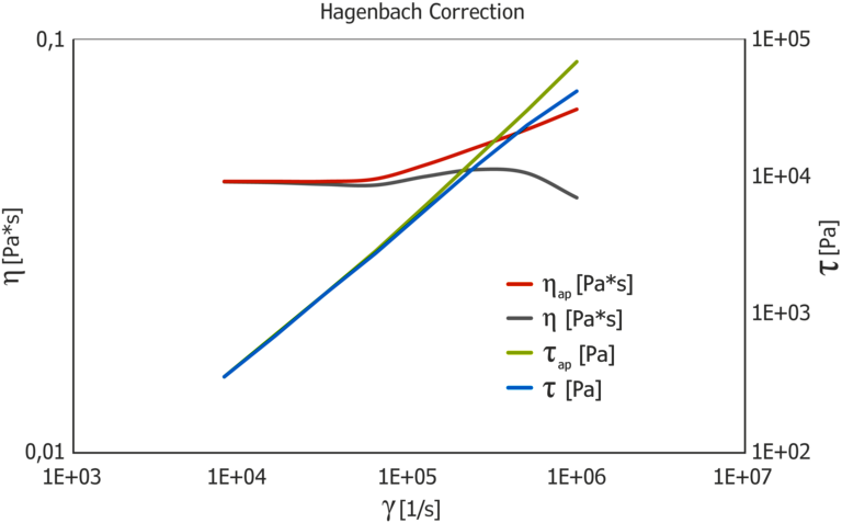
Due to the change in cross section between the test channel and capillary, there is a strong acceleration of the material entering the die. In the case of low-viscosity media such as, for example, emulsion paints, varnishes and oils, the pressure loss due to the acceleration work in relation to the viscous pressure loss is relatively large. Hagenbach correction takes this effect into account and eliminates it. For the correction, the density at the test temperature must be known.
The following example shows the effect of the Hagenbach correction compared to uncorrected data using the example of a paper coating ink.
For most thermoplastics, the Hagenbach correction is not necessary, because the increase in kinetic energy in relation to the pressure loss due to viscous flow is very small.
Due to the different requirements for the implementation of individual corrections, the corrections must be carried out in the correct order for physical reasons. The following listing indicates only the order and does not represent a weighting of their respective impact. It is a matter of judgment which corrections are actually necessary.
High viscous materials > ~ 1 Pas (e.g. plastic, rubber):
Low viscous materials < ~ 1 Pas (e.g. varnish, polymer solution):
In practice, for most of the high-viscosity materials, Bagley and Weißenberg-Rabinowitsch correction is used. In a high-pressure capillary rheometer with two test barrels, the necessary two tests can be carried out in one shot.